Algorithm and Data Structure Summary
算法与数据结构汇总
Big-O Concept
{O 上界} {Ω Omega 下界} {Θ Theta 上下界}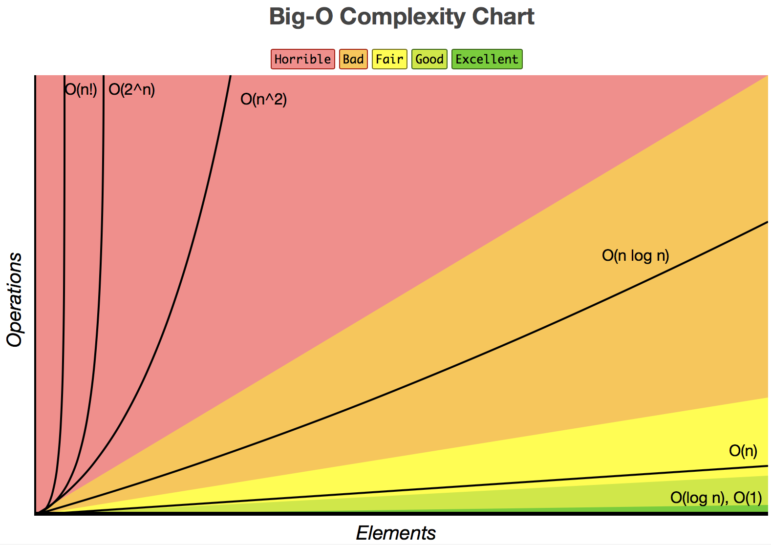
Sorting Algorithm Complexity

 (credit to: https://www.toptal.com/developers/sorting-algorithms/)
Data Structure 数据结构
array 数组
- 特性
- ordered
- random-access (constant O(1) time access)
- get_length - O(1)
- append_last - O(1)
dictionary 字典
key-value hashable
1 | # python |
1 | // swift |
linked list 链表
benefit: can add and remove items from the beginning of the list in constant time.
singly linked list 单向链表, doubly linked list 双向链表
- runer technique: iterate through the linked list with two pointers simultaneously (fast and slow)
1 | # python |
1 | // swift |
set 集合
unordered collecition of unique values
- dic 字典
- hashtable
1 | # python |
1 | // swift |
list 列表
stack queue priority queue heap
stack 栈
{LIFO}{push, pop, top, isEmpty}
1 | # python |
1 | // swift |
queue 队列
{FIFO}{enqueue, dequeue, front, rear, isEmpty}
- can be created in four ways:
- array - {dequeue in this struct takes O(n)}
- doubly linked list - {elements aren’t in contiguous blocks of memory. will increase access time}
- ring buffer - {fixed size}
- two stacks - {best}
1 | # python3 |
1 | // swift |
priority queue 优先队列
heap 堆
can also be developed in tree structure
[]
graph 图
{G = <V-vertex, E-edge>} {directed, undirected ,weighted, unweighted}
- complete graph 完全图
- dense graph 稠密图
- spares graph 稀疏图
- {表示方法: adjacency matrix邻接矩阵 - 适合稠密图 & adjacency lists邻接链表 - 适合稀疏图}
1 | # python |
tree 树
{|E| = |V| - 1}
- tree
- binary tree
- binary search tree (BST) 二叉查找树 {math.floor(logn) <= h <= n-1}
- balanced search tree 平衡查找树
- self-balancing 自平衡查找树
- AVL tree
- 每个节点的左右子树高度差不超过1
- red-black tree 红黑树
- 能容忍同一节点的一棵子树的高度是另一棵子树的两倍
- splay tree 分裂树
- AVL tree
- 允许单个节点中包含不只一个元素
- 2-3 tree
- 2-3-4 tree
- B tree
- self-balancing 自平衡查找树
- complete binary tree 完全二叉树
- heap (binary heaps) {complete binary tree}
- 可以用完全二叉树实现, 树的每一层都是满的,除了最后一层最右边元素可能缺位
- 父母优势, 每一个节点的键都要大于等于它子女的键
1 | 10 |
- Trie tree (prefix trees) 单词查找树
1
2
3
4
5root
/ \
T C
/ \ / \
R. O. A. O.
tree
1 | # python |
1 | // swift |
binary tree 二叉树
1 | # python |
1 | // swift |
1 | // swift |
Note: This BinaryTreeNode discription algorithm from Optimizing Collections
- tree traversal
- preorder (左中右)
- inorder (中左右)
- postorder (左右中)
1 | def preorder(tree): |
1 | // swift |
binary search tree (BST) 二叉查找树
math.floor(logn) <= h <= n-1
fast lookup, addition, and removal operations: O(logn)
- value of left child less than its parent
- value of right child greater than or equal to its parent
1 | # python |
1 | // swift |
AVL Tree
self-balancing binary search tree
- Rotations
- left
- right-left
- right
- left-right
1 | # python |
1 | // swift |
Brute Force 蛮力法
selection sort 选择排序
{无论什么情况排序速度一样快}
- 从第一个元素开始从它之后找最小的元素与之交换.
- Time complexity: {Average: Θ(n^2), Worse: O(n^2), Best: Ω(n^2)}
- Space complexity: {O(1)}
1 | def selection_sort(list): |
bubble sort 冒泡排序
{对于差不多排好序的速度很快,可以到达Ω(n)}
- 比较相邻元素并将最大的元素向后沉直到最后,重复这个步骤
- Time complexity: {Average: Θ(n^2), Worse: O(n^2), Best: Ω(n)}
- Space complexity: {O(1)}
1 | def bubble_sort(list): |
sequential search 顺序查找 线性算法
- Time complexity: {Average: Θ(n), Worse: O(n), Best: Ω(1)}
- Space complexity: {O(1)}
1 | def sequential_search(list, k): |
dfs 深度优先查找
- Time complexity: O(|V|+|E|) = O(b^{d})
- Space complexity: O(|V|)
1 | def dfs(graph, start): |
bfs 广度优先查找
- Time complexity: O(|V|+|E|) = O(b^{d})
- Space complexity: O(|V|) = O(b^{d})
1 | def bfs(graph, start): |
Decrease-And-Conquer 减治法
insertion sort 插入排序
{对于差不多排好序的速度很快,可以到达Ω(n)}
- 从第二个元素开始向前找到正确的位置插入
- Time complexity: {Average: Θ(n^2), Worse: O(n^2), Best: Ω(n)}
- Space complexity: {O(1)}
1 | def insetion_sort(list): |
shell sort 希尔排序
- 通过一个gap来左插入排序(常用方法是从len/2gap开始每次缩小2倍)
- Time complexity: {Average: Θ(n(logn)^2), Worse: O(n(logn)^2), Best: Ω(nlogn)}
- Space complexity: {O(1)}
1 | def shell_sort(list): |
generating permutations
- JohnsonTrotter
- Time complexity: O(n!)
binary search 折半查找
- Time complexity: {Average: Θ(logn), Worse: O(logn), Best: Ω(1)}
- Space complexity: {O(1)}
1 | def binary_search(sorted_list, target): |
quick select 快速选择
- 寻找第k个最小元素,通过划分来实现
- Time complexity: {Average: Θ(n), Worse: O(n^2), Best: Ω(n)}
- Space complexity: O(1)
1 | def quick_select_m(list, start, end, k_th_min): |
Divide-And-Conquer 分治法
分解问题,求解子问题,合并自问题的解
T(n) = aT(n/b) + f(n) {a个需要求解的问题,问题被分成b个,f(n)的分解合并时间消耗}
T(n) = O(n^d) if a < b^d or O(n^dlogn) if a = b^d or O(n^log_b(a)) if a > b^d
merge sort 归并排序
{除了heapsort以外唯一BestAveWorst全是O(nlogn)排序算法}
- 两种实现方法(自顶向下-递归, 自底向上-循环)
- Time complexity: {Average: Θ(nlogn), Worse: O(nlogn), Best: Ω(nlogn)}
- Space complexity: {O(n)}
1 | def merge_sort(list): |
quick sort 快速排序
{pivot的选择对于算法效率至关重要}
- 不断选择pivot来将元素划分到它的左右来实现
- Time complexity: {Average: Θ(nlogn), Worse: O(n^2), Best: Ω(nlogn)}
- Space complexity: {O(nlogn)}
- pivot每次选第一个在已经排好序的数组上时间效率是O(n^2)
- 优化方法
- 使用随机pivot, 平均划分pivot, 快排好后使用插入排序
- 优化方法
1 | def quick_sort_m(list, start, end): |
Transform-And-Conquer 变治法
- 预排序解决问题
- 检查数组中元素的唯一性
- 算法数组的模式 (一个数组中最多的元素)
heap sort 堆排序
- 先构建一个堆, 不断的删除最大键,
- Time complexity: {Average: Θ(nlogn), Worse: O(nlogn), Best: Ω(nlogn)}
- Space complexity: {O(1)}
1 | import heapq |
problem reduction 问题简化
{已有一种方法求其他问题}
- lcm(m, n) * gcd(m, n) = m * n {lcm: 最小公倍数, gcd: 最大公约数}
- 求一个函数的最小值, 可以求一个函数负函数的最大值的负数
hash table 散列表
- 需要把键在hash table 中尽可能均匀分布
- 平均插入,删除, 查找效率都是 O(1), 当最坏情况全部冲突到一个位置时候,退化到 O(n)
- open hasing, also: separate chaining 分离链 开hash
- closed hashing 闭hash
- double hashing
- rehasing
B-tree B树
Dynamic Programming (DP) 动态规划
- 与其对交叠的子问题一次又一次地求解,还不如对每个较小的子问题只求解一次并把结果记录在表中。 (对具有交叠子问题的问题进行求解的技术)
- 类似斐波那契数
coins_row problem (求互不相临的最大金币总金额)
- Time complexity: O(n), Space complexity: O(n)
1 | def coin_row(coins): |
change_making problem
- Time complexity: O(mn), Space complexity: O(n)
1 | def change_making(coins, change): |
knapsack problem 背包问题
- Time complexity: O(nW), Space complexity: O(nW)
- #TODO
memory function 记忆功能
TODO
Greedy Technique 贪婪技术
Prim
- 构造最小生成树算法
- 先随机选一个点,每次扩展新的点使得这个新的点到已有点的距离最短,直到添加完所有顶点
1 | # TODO (heaven) |
Kruskal
- 构造最小生成树算法
- 先按照权重将边进行排序,然后不断把边加入子图,如果加入此边会产生回路,则天国,直到完成
1 | # TODO (heaven) |
Dijkstra
- 单起点最短路径问题
1 | # TODO (heaven) |
Bit Operation
- get bit
1 | def is_git_i_1(num, i): |
- set bit
1 | def set_bit(num, i): |
- clear bit
1 | def clear_bit(num, i): |
- update bit
1 | def update_bit(num, i, v): |
How To Optimaize the Algorithm
Optimaize & Solve Technique
- Look for BUD
- Bottlenecks
- Unnecessary work
- Duplicated work
- DIY (Do It Yourself)
- Simplify and Generalize
- Base Case and Build (always use for recursion)
- like for generate permutations
1
2
31 Case "a" --> {"a"}
2 Case "ab" --> {"ab", "ba"}
3 Case "abc" --> {"cab", "acb", "abc", "cba", "bca", bac"}
- like for generate permutations
- Data structure brainstorm
- hash
- heap
- tree
- Look for BUD
Consider the BCR (Best Conceivable Runtime)
- The BCR is the best runtime you could conceive of a solution to a problem having.You can easily prove that there is no way you could beat the BCR.
Good coding looks like
- correct
- efficient
- simple
- readable
- maintainable
- use data structures generously
- appropriate code resue
- modular
- flexible and robust
- error checking
Power Table of 2
| 2^ | = | approximation | approximate to |
|---|---|---|---|
| 7 | 128 | ||
| 8 | 256 | ||
| 10 | 1024 | one thousand | 1K |
| 16 | 65536 | 64K | |
| 20 | 1048576 | one million | 1MB |
| 30 | 1073741824 | one billion | 1GB |
| 32 | 4294967296 | 4GB | |
| 40 | 1099511627776 | one trillion | 1TB |
Author: Min Gao
如需转载或引用, 请标注出处。